Comparing Two Soundings

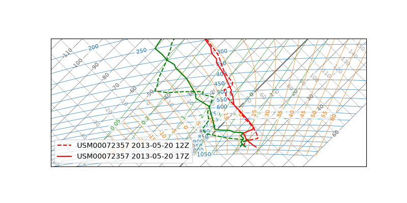
Two ascents from the same station on the same day, each a sounding, framed together so the change between them is the only thing that moves.

Norman, Oklahoma on 2013-05-20: the 12Z ascent, and the 17Z special released about three hours before the Moore EF5 tornado. Over those five hours the cap erodes from -271 J/kg to nothing while CAPE nearly triples. Everything that changed between them lies in the lower troposphere, so fit is clamped to that layer: both ascents run out the top of the view near 300 hPa, and neither one’s own data decides the frame the comparison is read in.

from __future__ import annotations

from typing import TYPE_CHECKING

import matplotlib.pyplot as plt

from tephpy import samples

if TYPE_CHECKING:
    from matplotlib.figure import Figure


def main() -> Figure:
    """Overlay the 12Z and 17Z ascents.

    Returns
    -------
    matplotlib.figure.Figure
        The composed figure.
    """
    morning = samples.sounding("norman-12z")
    afternoon = samples.sounding("norman-17z")
    fig, ax = plt.subplots(figsize=(8.0, 4.0), subplot_kw={"projection": "tephigram"})
    ax.fit(morning, afternoon, pressure=(950.0, 300.0))
    ax.plot_sounding(morning, linestyle="--")
    ax.plot_sounding(afternoon)
    # The default "best" placement lands on the data where the two traces
    # converge near the top of the clamped view; the lower left stays open.
    ax.legend(loc="lower left")
    return fig

Saving the Figure

The diagram is drawn as vectors, so it saves at publication quality:

fig.savefig("sounding-comparison.pdf")

It is shown rather than run, so that browsing the gallery writes no files.

if __name__ == "__main__":
    main()
    plt.show()

🏷 Tags: overlay, sounding