Analyse a Sounding

Estimated reading time: 6 minutes

Your First Tephigram drew an ascent and named the lines on it. This page asks the question a forecaster asks next: was this atmosphere capable of a storm? By the end you will have lifted a parcel through it, shaded the two energies that answer the question, and put the numbers on the figure.

It continues from the same ascent, so if you have just come from that page you know this sounding. If you have not, the first block below is all you missed.

Lift a Parcel

Take the air at the surface and imagine pushing it upward. It cools as it rises, and if it ends up warmer than its surroundings it keeps going by itself — that is a storm getting started. calc.parcel_path(...) computes the path that parcel takes:

import matplotlib.pyplot as plt

import tephpy
from tephpy import samples

snd = samples.sounding("norman-12z")

fig, ax = plt.subplots(subplot_kw={"projection": "tephigram"})
ax.plot_sounding(snd)
parcel = tephpy.calc.parcel_path(snd, label="surface parcel")
ax.plot_profile(parcel, color="k", linestyle="--")
ax.legend()

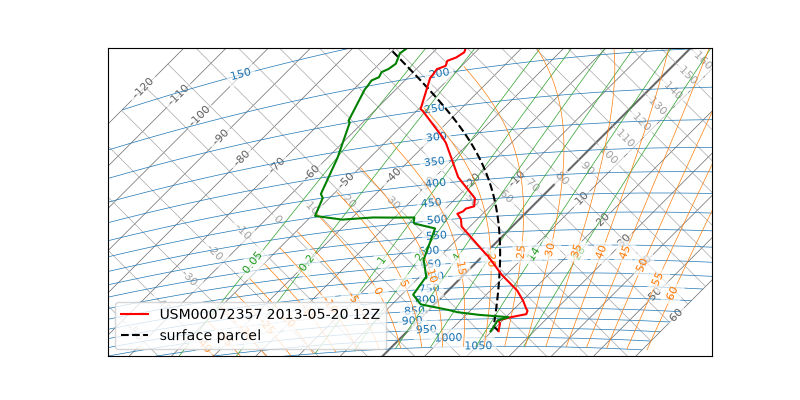
The dashed black line is the parcel. It leaves the surface along a straight dry adiabat and bends where it becomes saturated — cloud base, at 939 hPa for this ascent, which is close enough to the ground that the straight section is short. Above the bend the parcel is condensing its water and releasing latent heat, so it cools more slowly. That corner is Normand’s point, and Parcel Ascent and Normand’s Point derives it.

Compare the dashed line with the red one. Low down the parcel sits on the cool side of it — it would sink back if you let go. Higher up it crosses over and stays warmer to well above 300 hPa. Those two regions are the answer to the question this page opened with, and the next block makes them visible.

Shade the Two Energies

Where the parcel is colder than its environment, lifting it costs energy: that is convective inhibition, the lid. Where it is warmer, the atmosphere gives energy back: that is convective available potential energy, the fuel.

Both are areas on this diagram — which is a property of the tephigram’s axes rather than a convention, and Why the Axes Are Rotated explains why:

fig, ax = plt.subplots(subplot_kw={"projection": "tephigram"})
ax.plot_sounding(snd)
ax.plot_profile(parcel, color="k", linestyle="--")
ax.shade_cape(snd, parcel)
ax.shade_cin(snd, parcel)
ax.legend()

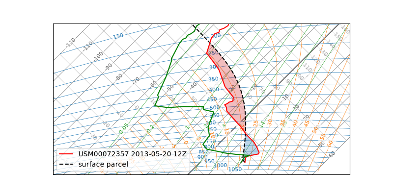
Red is CAPE and blue is CIN. Read them the way a forecaster does: a large red area means a lot of energy available to a storm, and a large blue one means something has to lift the air through the lid before any of it is released. This sounding has both — which is what made the day it was taken from notable.

Put the Numbers On

Areas are for reading by eye. For the numbers, calc.indices(...) computes ten of them and ax.annotate_indices(...) puts them in a panel beside the diagram:

fig, ax = plt.subplots(subplot_kw={"projection": "tephigram"})
ax.plot_sounding(snd)
ax.plot_profile(parcel, color="k", linestyle="--")
ax.shade_cape(snd, parcel)
ax.shade_cin(snd, parcel)
ax.annotate_indices(tephpy.calc.indices(snd))
ax.legend()

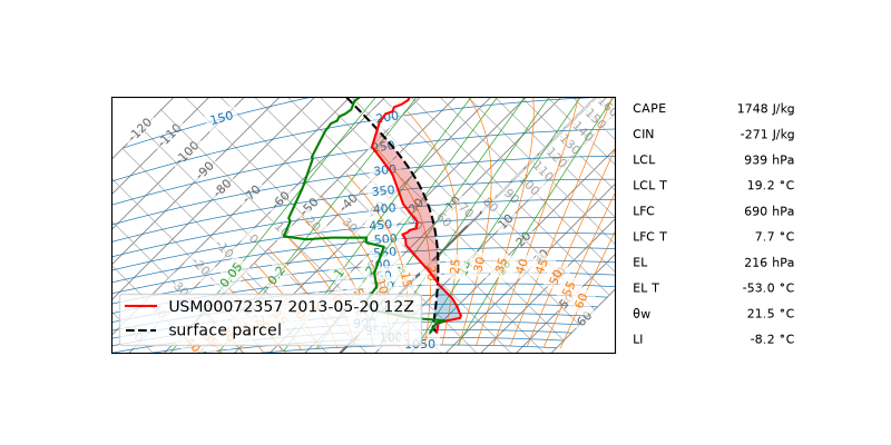
That panel is a rendering of an object you can read yourself. calc.indices(...) returns a SoundingIndices, whose ten fields — cape, cin, the pressure and temperature of each of the three levels, theta_w and lifted_index — are pint quantities you can pull out and use like any other number.

The panel names the two shaded areas in joules per kilogram, and the levels the construction passed through on its way: cloud base (the LCL), the level of free convection where the parcel finally became buoyant, and the equilibrium level where it ran out. Some of those fields can be NaN, and that is an answer rather than a failure: a parcel that never becomes buoyant has no level of free convection, so the LFC and EL rows report NaN rather than a number. The two energies are different — CAPE and CIN are 0 J/kg when there is nothing to report, never NaN, so a zero there means a real absence rather than a gap.

You now have the whole analysis on one figure: the environment, the parcel, the energies as areas, and the numbers.

Where to Go Next

The gallery shows this same analysis as a finished example, alongside what else the package draws. Parcel Ascent and Normand’s Point derives the construction rather than driving it, and Emphasise a Reference Isopleth marks the reference lines a forecaster reads against.